How to performs cell based segmentation with the watershed algorithm

In this notebook we will show you how to performs watershed segmentation of a grayscale image representing a biological tissue at cell level, i.e. where the signal is delimitatin cells. We will details each step and thus use functions from the algorithms module.

This guide is not intended for nuclei detection, although it could work with some minor adjustments, there are probably more robust ways of performing this task.

%matplotlib inline
import numpy as np
from timagetk.algorithms.connexe import connected_components
from timagetk.algorithms.exposure import global_contrast_stretch
from timagetk.algorithms.linearfilter import linearfilter
from timagetk.algorithms.regionalext import regional_extrema
from timagetk.algorithms.watershed import watershed
from timagetk.components.spatial_image import SpatialImage
from timagetk.io import imread

/builds/J-gEBwyb/0/mosaic/timagetk/src/timagetk/components/labelled_image.py:31: TqdmWarning: IProgress not found. Please update jupyter and ipywidgets. See https://ipywidgets.readthedocs.io/en/stable/user_install.html
  from tqdm.autonotebook import tqdm

The image should be a 2D or 3D single channel grayscale image of a cellular tissue.

from timagetk.io.image import _image_from_url
tmp_path = _image_from_url('https://zenodo.org/record/7151866/files/p58-t0-imgFus.inr.gz',
                           hash_value='48f6f9924289037c55ea785273c2fe72', hash_method='md5')
image = imread(tmp_path)

  0%|          | 0.00/40.5M [00:00<?, ?B/s]

  3%|▎         | 1.06M/40.5M [00:00<00:03, 10.6MB/s]

  5%|▌         | 2.12M/40.5M [00:00<00:03, 10.7MB/s]

  8%|▊         | 3.16M/40.5M [00:00<00:03, 10.5MB/s]

 10%|█         | 4.22M/40.5M [00:00<00:03, 10.5MB/s]

 13%|█▎        | 5.41M/40.5M [00:00<00:03, 10.9MB/s]

 16%|█▌        | 6.47M/40.5M [00:00<00:03, 10.7MB/s]

 19%|█▊        | 7.53M/40.5M [00:00<00:03, 10.7MB/s]

 22%|██▏       | 8.94M/40.5M [00:00<00:02, 11.6MB/s]

 25%|██▍       | 10.1M/40.5M [00:00<00:02, 11.1MB/s]

 28%|██▊       | 11.2M/40.5M [00:01<00:02, 11.1MB/s]

 30%|███       | 12.2M/40.5M [00:01<00:02, 10.9MB/s]

 33%|███▎      | 13.3M/40.5M [00:01<00:02, 11.0MB/s]

 36%|███▌      | 14.4M/40.5M [00:01<00:02, 10.8MB/s]

 38%|███▊      | 15.5M/40.5M [00:01<00:02, 10.8MB/s]

 41%|████      | 16.6M/40.5M [00:01<00:02, 10.9MB/s]

 44%|████▎     | 17.7M/40.5M [00:01<00:02, 10.9MB/s]

 46%|████▋     | 18.8M/40.5M [00:01<00:02, 11.0MB/s]

 49%|████▉     | 19.8M/40.5M [00:01<00:02, 10.8MB/s]

 52%|█████▏    | 20.9M/40.5M [00:02<00:01, 10.7MB/s]

 55%|█████▍    | 22.1M/40.5M [00:02<00:01, 11.1MB/s]

 57%|█████▋    | 23.2M/40.5M [00:02<00:01, 10.9MB/s]

 60%|█████▉    | 24.2M/40.5M [00:02<00:01, 10.5MB/s]

 62%|██████▏   | 25.2M/40.5M [00:02<00:01, 10.6MB/s]

 65%|██████▍   | 26.3M/40.5M [00:02<00:01, 9.97MB/s]

 67%|██████▋   | 27.3M/40.5M [00:02<00:01, 10.2MB/s]

 70%|██████▉   | 28.3M/40.5M [00:02<00:01, 10.0MB/s]

 74%|███████▍  | 29.9M/40.5M [00:02<00:00, 11.6MB/s]

 78%|███████▊  | 31.7M/40.5M [00:02<00:00, 13.4MB/s]

 83%|████████▎ | 33.7M/40.5M [00:03<00:00, 15.4MB/s]

 87%|████████▋ | 35.2M/40.5M [00:03<00:00, 15.1MB/s]

 91%|█████████ | 36.8M/40.5M [00:03<00:00, 15.6MB/s]

 95%|█████████▍| 38.4M/40.5M [00:03<00:00, 15.8MB/s]

 99%|█████████▊| 39.9M/40.5M [00:03<00:00, 15.2MB/s]

40.5MB [00:03, 12.0MB/s]                            

from timagetk.visu.stack import orthogonal_view
orthogonal_view(image)

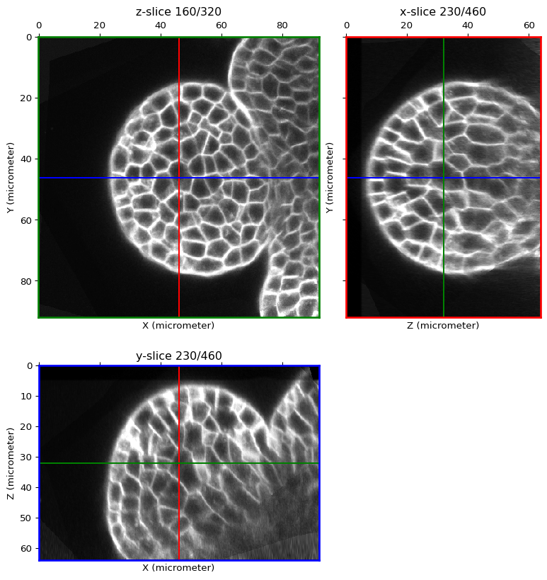
Pre-processing

Optional - Intensity rescaling

It may be useful to start with intensity rescaling since the image contrast might not be homogeneous or the intensity range not optimal (e.g. ranging in [15, 200] on a signed 8bit image that have a [0, 255] range)

image = global_contrast_stretch(image)

orthogonal_view(image)

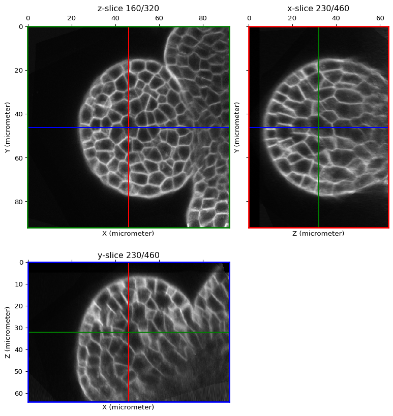
Linear filtering using Gaussian smoothing

To smooth out the noise in the image, we strongly advise to performs a gaussian smoothing prior to the following steps.

image = linearfilter(image, method="smoothing", sigma=1.0, real=True)
print(image.shape)

(320, 460, 460)

orthogonal_view(image)

Processing

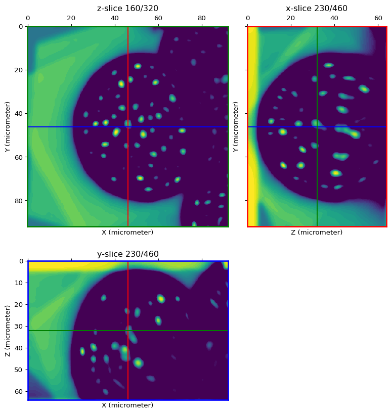
Local minima detection

This is the most critical step with the choice of a good h-minima value.

from timagetk.array_util import guess_intensity_threshold
th = guess_intensity_threshold(image)
print(f"Automatic threshold value: {th}")

Automatic threshold value: 62.400000000000006

hmin = int(round(th)/2)
print(f"H-minimum value for detection of local minima: {hmin}")
ext_img = regional_extrema(image, height=hmin, method='minima')

H-minimum value for detection of local minima: 31

orthogonal_view(ext_img, cmap='viridis', val_range=[0, hmin])

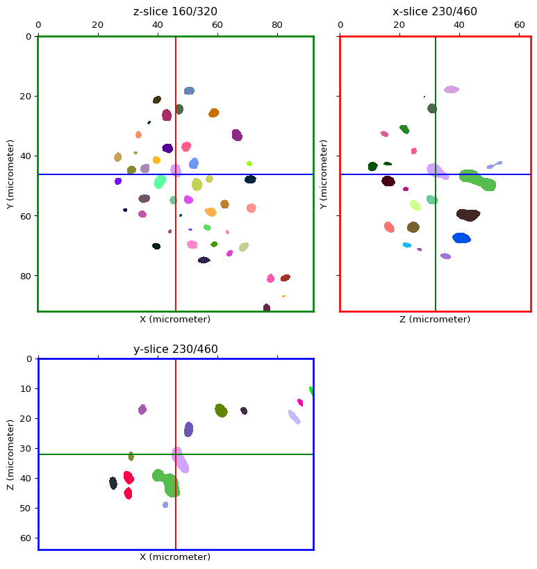
Connected component labelling of detected local minima

This step is labelling each detected local minima with a unique id to generate a seed image.

seeds_image = connected_components(ext_img, low_threshold=1, high_threshold=hmin)

n_seeds = len(np.unique(seeds_image)) - 1  # '0' is in the list!
print("Detected {} seeds!".format(n_seeds))

Detected 202 seeds!

orthogonal_view(seeds_image, cmap='glasbey', val_range=[1, n_seeds])

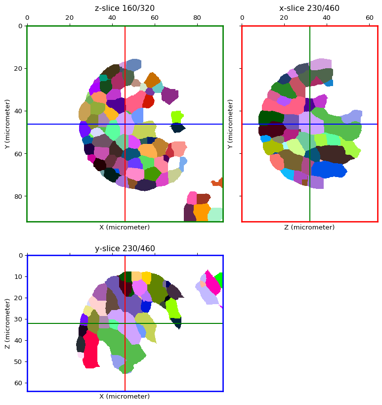
Seeded watershed

The previously detected seeds are now used by the watershed algorithm to “flood” the cells.

label_image = watershed(image, seeds_image, method="first")

orthogonal_view(label_image, cmap='glasbey', val_range=[1, n_seeds])